What You'll Learn
- Know each activation's formula, range and derivative
- Understand saturation and the resulting vanishing-gradient problem
- Recognise the dying-ReLU problem and how Leaky/Parametric ReLU fixes it
- Use softmax to turn scores into a probability distribution for multi-class output
- Choose the right activation per layer (hidden vs. output)
Prerequisites: Module 3 (Neural Network Foundations). You should already be comfortable with a neuron's weighted sum \( z = w\cdot x + b \) and how a network stacks neurons into layers before starting here.
Binary Step & Linear
An activation function takes a neuron's weighted sum \( z = w\cdot x + b \) and decides what the neuron outputs. Without one, a neuron can only compute a straight line. The whole point of the functions in this module is to inject non-linearity — the ingredient that lets a network learn curved, complicated decision boundaries. We begin with the two simplest cases, both of which turn out to be inadequate as hidden-layer activations.
Binary Step
The binary step function fires only when the input clears a threshold \( t \):
\[ f(x)=\begin{cases}0 & x < t \\[4pt] 1 & x \ge t\end{cases} \]
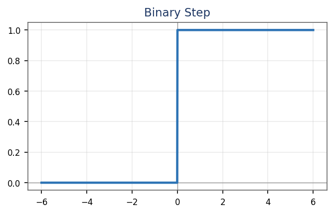
With a step activation a neuron becomes a perceptron: it outputs 1 or 0 depending purely on whether \( w\cdot x + b \) is positive or negative (binary classification). It is beautifully interpretable, but it has two fatal flaws: it gives no multi-value outputs (so no multi-class problems), and its gradient is zero everywhere — so backpropagation has nothing to work with.
Linear (Identity)
The linear, or identity, activation simply scales its input (with slope \( a \)):
\[ f(x) = a\,x \]
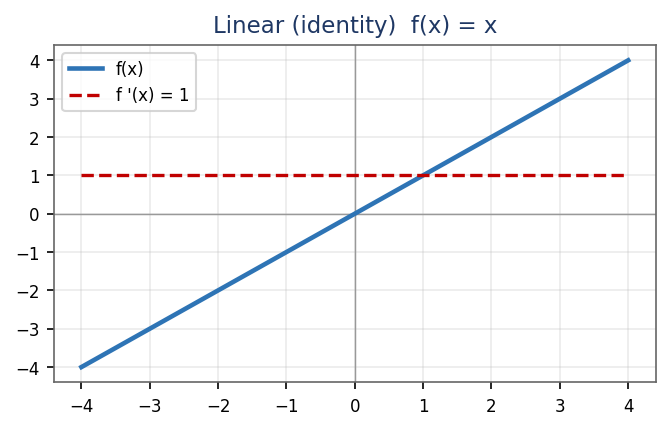
Also called “no activation” — it passes the weighted sum through unchanged, which is equivalent to plain linear regression. Its derivative is the constant \( a \), so the gradient carries no information about the input — every input pushes the weights the same way. Worse, stacking linear layers is pointless: a linear function of a linear function is still linear, so any number of linear layers collapses to a single layer. That makes the linear activation unusable as a hidden activation.
Advantages & Limitations
- Step — advantage: maximally simple and interpretable (a clean yes/no perceptron).
- Step — limitation: zero derivative everywhere and no multi-value output, so it cannot be trained by backpropagation and cannot do multi-class problems.
- Linear — advantage: unbounded output, fine for the output layer of a regression model.
- Linear — limitation: constant gradient \( f'(x)=a \) and layer-collapse make it worthless as a hidden activation.
Non-linear activation functions solve both problems: they make backpropagation possible and let us stack many layers. The main ones — Sigmoid, Tanh, ReLU, Leaky ReLU, Softmax and Swish — are covered next.
Sigmoid (Logistic)
The sigmoid, or logistic function, is the classic smooth switch. Its formula and range are:
\[ \sigma(x) = \frac{1}{1 + e^{-x}}, \qquad \text{range: } (0,\,1) \]
and its derivative has an elegant closed form:
\[ \sigma'(x) = \sigma(x)\,\bigl(1 - \sigma(x)\bigr) \]
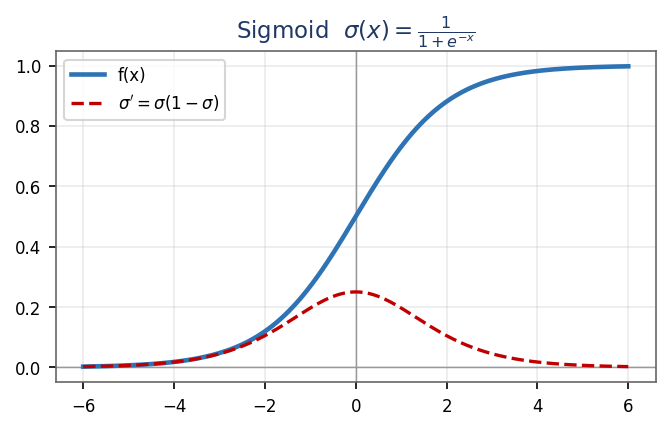
It is S-shaped (the “logistic curve”): a large positive input maps to nearly 1 (neuron fires), a large negative input to nearly 0, and an input near 0 to about 0.5 (a fuzzy region). Because the output always lies in \( (0,\,1) \), it reads naturally as a probability — which is why sigmoid is the standard activation for the output of a binary classifier.
Advantages & Limitations
- Advantage: smooth, differentiable everywhere, output bounded in \( (0,\,1) \) as a natural probability, and a simple derivative \( \sigma(1-\sigma) \).
- Limitation — vanishing gradient: it saturates at both ends — for \( x > 3 \) or \( x < -3 \) the curve flattens and \( \sigma'(x) \to 0 \), so gradients vanish and deep layers stop learning.
- Limitation: the output is not zero-centered (all outputs are positive), which makes training slower and less stable; and \( e^{x} \) is computationally expensive.
Saturation: a node is saturated when most of its outputs sit at the bounds of the activation function (near 0 or 1). Saturated neurons “kill” the gradient.
Tanh
The hyperbolic tangent is a rescaled sigmoid. Its formula and range are:
\[ \tanh(x) = \frac{2}{1 + e^{-2x}} - 1, \qquad \text{range: } (-1,\,1) \]
and its derivative is:
\[ f'(x) = 1 - \tanh^{2}(x) \]
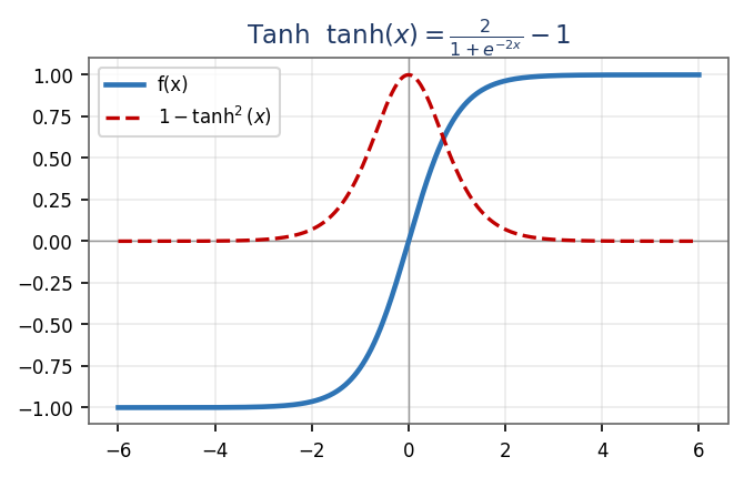
Tanh has the same S-shape as sigmoid, but it is zero-centered: negative inputs map to negative outputs and positive to positive. That symmetry is a genuine advantage over sigmoid — hidden-layer means stay near 0, which centers the data and makes learning in the next layer easier. In practice tanh is always preferred over sigmoid for hidden layers: both saturate, but tanh is zero-centered and its gradients are not restricted to one direction.
Advantages & Limitations
- Advantage: zero-centered output with a steeper gradient than sigmoid, so it typically trains faster.
- Limitation: it still saturates at both extremes, so it too causes vanishing gradients in deep networks; and \( e^{x} \) is still computationally expensive.
ReLU — Rectified Linear Unit
The Rectified Linear Unit is the default hidden activation of modern deep learning. Its formula is almost embarrassingly simple:
\[ f(x) = \max(0,\,x) \]
and its derivative is a clean 0/1 switch:
\[ f'(x) = \begin{cases}0 & x < 0 \\[4pt] 1 & x > 0\end{cases} \]
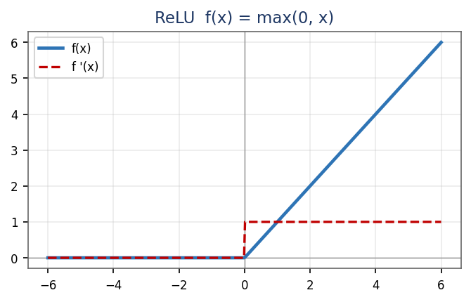
ReLU looks linear, but it is genuinely non-linear because of the kink at 0, and it has a usable derivative, so backpropagation works while staying extremely cheap to compute. It also produces sparse activation: any neuron whose weighted sum is negative outputs exactly 0 (like a Boolean gate), so not all neurons fire at once, which is efficient and often helpful. In practice it converges roughly \( 6\times \) faster than sigmoid/tanh.
Advantages & Limitations
- Advantage: does not saturate for positive \( x \), is very computationally efficient, gives sparse activations, and is the recommended default for MLPs and CNNs.
- Limitation: not zero-centered, and not differentiable exactly at \( x = 0 \).
- Limitation — the “dying ReLU”: a neuron whose weighted sum stays negative outputs 0 forever. Since the gradient there is also 0, its weights never update — the neuron dies permanently, especially with a high learning rate or unlucky initialization.
Leaky & Parametric ReLU
Leaky ReLU is a one-line patch for the dying-ReLU problem: give the negative side a small non-zero slope \( \alpha \) (typically 0.01):
\[ f(x) = \begin{cases}x & x > 0 \\[4pt] \alpha\,x & x \le 0\end{cases} \qquad (\alpha \text{ small, e.g. } 0.01) \]
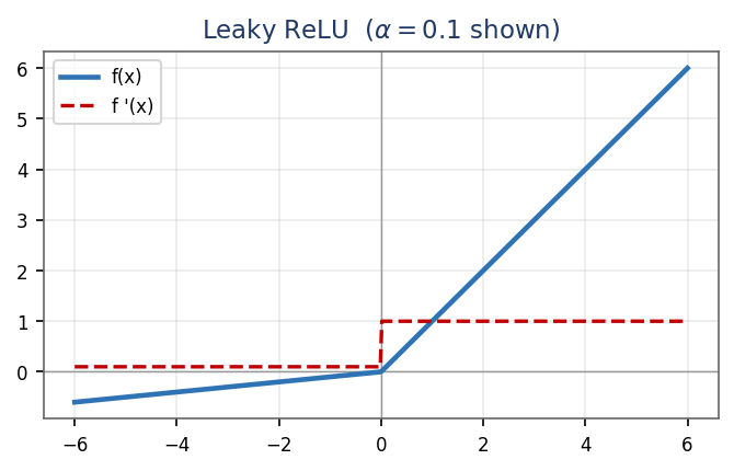
Because the negative side now has a small but non-zero slope, the gradient is never exactly zero (it is \( \alpha \) for \( x \le 0 \) and 1 for \( x > 0 \)), so a neuron can always nudge its weights back into a useful region — neurons can't die. Parametric ReLU (PReLU) uses the same formula but makes \( \alpha \) a learnable parameter: backpropagation finds the most appropriate value of \( \alpha \) for the task.
Advantages & Limitations
- Advantage: keeps all of ReLU's speed and non-saturation but removes the dying-ReLU problem — the gradient never vanishes on the negative side, so backpropagation works even for negative inputs.
- PReLU advantage: the network tunes \( \alpha \) itself, adapting the negative slope to the data.
- Limitation: predictions may be inconsistent for negative inputs, and the tiny negative-side gradient makes learning of those weights slow.
Softmax (Normalized Exponential)
Softmax is the output-layer activation for multi-class classification. For a vector of \( K \) real scores \( z \), the \( i \)-th output is:
\[ \text{softmax}(z_i) = \frac{e^{z_i}}{\sum_{j} e^{z_j}} \]
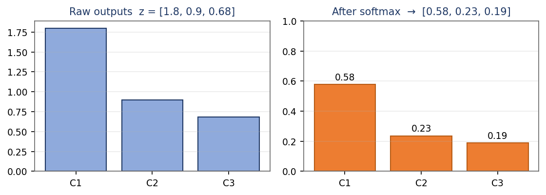
Softmax turns \( K \) arbitrary real scores into a proper probability distribution: every output lies in \( (0,\,1) \) and all \( K \) outputs sum to exactly 1. This fixes the problem raw scores have (e.g. outputs 0.8, 0.9, 0.7 do not sum to 1, so they aren't comparable probabilities). It behaves like a combination of multiple sigmoids, making it the natural activation at the output layer for multi-class classification, where each output reads as “the probability this input belongs to class \( i \).”
Cross-link: numerical stability
Module 2 covered the numerically-stable version of softmax — subtract the maximum score from every \( z_i \) before exponentiating, i.e. \( \text{softmax}(z_i) = \dfrac{e^{\,z_i - \max_k z_k}}{\sum_{j} e^{\,z_j - \max_k z_k}} \). The result is identical, but it prevents \( e^{x} \) from overflowing on large scores.
Swish
Swish is a smooth, self-gated activation — the input multiplied by its own sigmoid:
\[ \text{Swish}(x) = x\,\sigma(x) = \frac{x}{1 + e^{-x}} \]
Being built from the sigmoid, its derivative is smooth and non-monotonic, with the compact form \( \text{Swish}'(x) = \sigma(x) + x\,\sigma(x)\bigl(1 - \sigma(x)\bigr) \).
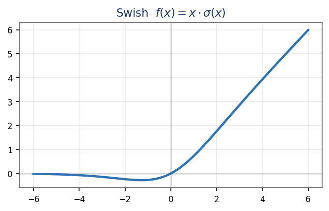
Developed by Google, Swish matches or outperforms ReLU on very deep networks (depth \( > 40 \) layers) for hard tasks such as image classification and machine translation. Its key structural difference from ReLU is smoothness: it does not abruptly change direction at \( x = 0 \) — it bends smoothly below zero and back up. Small negative values are kept (they may still carry useful pattern information) while large negative values are driven toward 0 for sparsity — a win-win.
Advantages & Limitations
- Advantage: smooth (no sharp corner), keeps small negative values, and often outperforms ReLU on very deep networks and hard tasks.
- Limitation: more expensive than ReLU (it computes a sigmoid), with gains that mainly appear once the network is very deep.
All Functions at a Glance
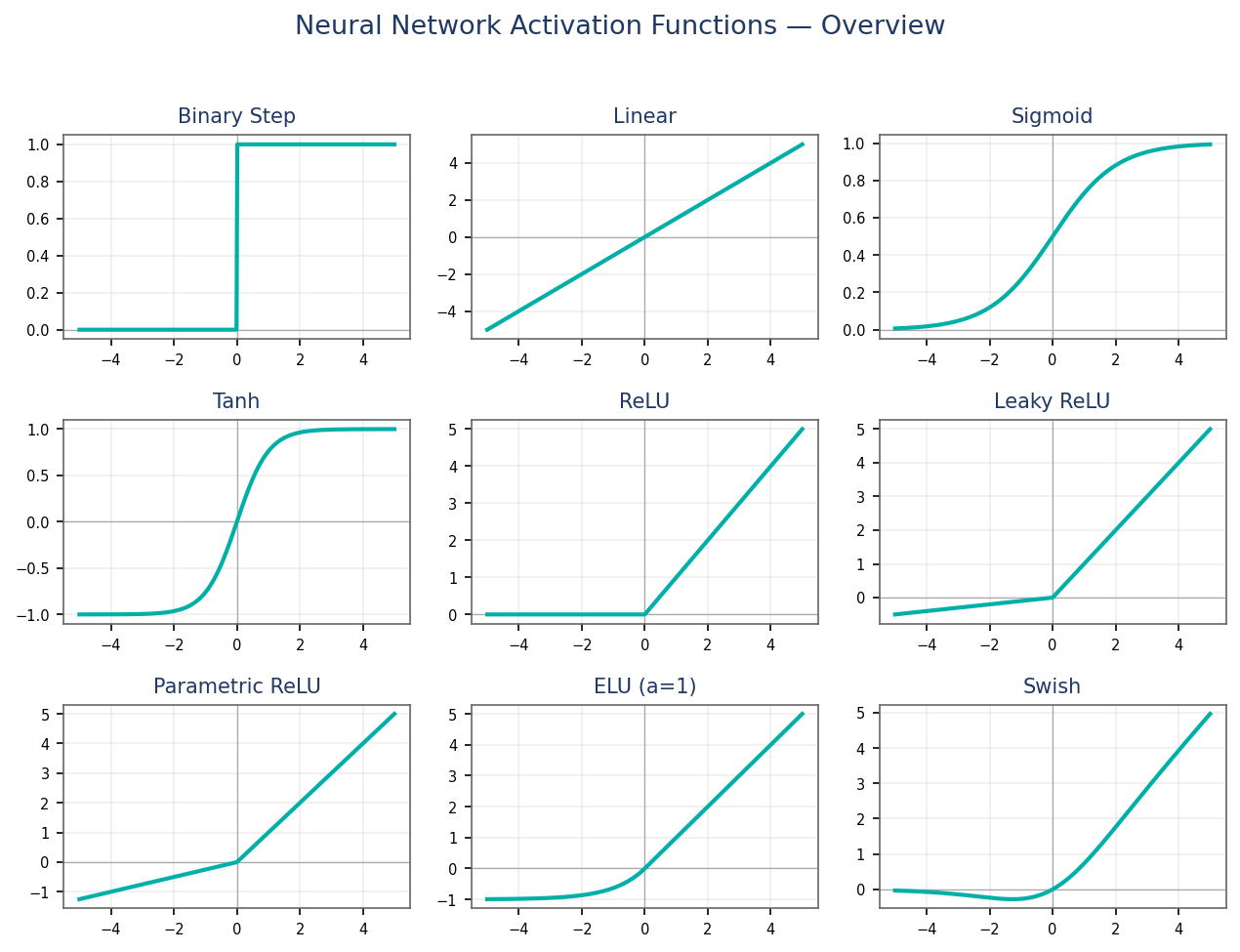
Seen together, the functions split cleanly into two families. The saturating functions — step, sigmoid and tanh — flatten out at both extremes, so their derivatives fall to nearly 0 for large \( |x| \) and gradients vanish in deep networks. The ReLU family — ReLU, Leaky/Parametric ReLU, and (smoothly) Swish — does not saturate on the positive side: the curve keeps climbing, so the gradient stays healthy no matter how large the input grows.
How to Choose the Right Activation
You do not have to agonise over this in practice. A handful of rules of thumb cover almost every network you will build:
Rules of thumb
- Start with ReLU in the hidden layers — switch to something else only if results aren't optimal.
- Use ReLU and its variants only in the hidden layers.
- Avoid sigmoid and tanh in the hidden layers of deep nets — they saturate and cause vanishing gradients during training.
- Use Swish for very deep networks (\( > 40 \) layers).
- Hidden layers almost always share the same activation, and it must be differentiable for backpropagation.
Output layer — choose by problem type
| Problem type | Output activation |
|---|---|
| Regression | Linear (or ReLU if output \( \ge 0 \)) |
| Binary classification | Sigmoid / Logistic |
| Multi-class classification | Softmax |
| Multi-label classification | Sigmoid (per label) |
Hidden layers — choose by architecture
| Architecture | Hidden activation |
|---|---|
| Multilayer Perceptron (MLP) | ReLU |
| Convolutional Neural Network (CNN) | ReLU |
| Recurrent Neural Network (RNN) | Tanh and/or Sigmoid |
When selecting an activation function, always consider the problems it might face: vanishing and exploding gradients.
Summary — Equations & Derivatives
Every activation from this module, its formula and its derivative in one place:
| Activation | Function \( f(x) \) | Derivative \( f'(x) \) |
|---|---|---|
| Linear | \( f(x) = ax + c \) | \( f'(x) = a \) |
| Sigmoid | \( f(x) = \dfrac{1}{1 + e^{-x}} \) | \( f'(x) = f(x)\bigl(1 - f(x)\bigr) \) |
| Tanh | \( f(x) = \dfrac{2}{1 + e^{-2x}} - 1 \) | \( f'(x) = 1 - f(x)^{2} \) |
| ReLU | \( f(x) = \begin{cases}0 & x<0\\ x & x\ge 0\end{cases} \) | \( f'(x) = \begin{cases}0 & x<0\\ 1 & x\ge 0\end{cases} \) |
| Leaky / Parametric ReLU | \( f(x) = \begin{cases}\alpha x & x<0\\ x & x\ge 0\end{cases} \) | \( f'(x) = \begin{cases}\alpha & x<0\\ 1 & x\ge 0\end{cases} \) |
| Softmax | \( \dfrac{e^{z_i}}{\sum_{j} e^{z_j}} \) | outputs a probability vector (sums to 1); used with cross-entropy loss |
Key takeaways
- Activation functions introduce non-linearity — without them any network collapses to a single linear layer.
- They must be differentiable so backpropagation can adjust the weights.
- ReLU is the default for hidden layers; sigmoid/softmax for classification outputs; linear for regression outputs.
- Watch out for vanishing gradients (saturating functions) and dying neurons (plain ReLU).
Exercises — Answer Key
Work each one on paper before opening the solution — plugging numbers through these formulas once is worth ten readings. Part A drills each activation; Part B tests comparison and design judgement.
Binary Step
A neuron has weights \( w = [1,\,-2] \), input \( x = [2,\,1] \), bias \( b = 1 \), and threshold \( t = 0 \). Compute the weighted sum \( z \) and the step output \( f(z) \). Does the neuron fire?
\[ z = (1)(2) + (-2)(1) + 1 = 2 - 2 + 1 = 1 \]
Since \( 1 \ge 0 \) (the threshold), the step function gives \( f(1) = 1 \).
Yes — the neuron fires.
Linear
For \( f(x) = 0.5x \) and input \( z = 4 \): what is the output, and what is \( f'(4) \)? Why is a constant derivative useless for backpropagation?
\[ f(4) = 0.5 \times 4 = 2, \qquad f'(x) = 0.5 \text{ for every } x, \text{ so } f'(4) = 0.5 \] The derivative is a constant, unrelated to the input. Backpropagation relies on the gradient telling each weight how the input affects the loss — but a constant derivative carries no information about the input, so it cannot guide learning, and stacked linear layers collapse into one.
Sigmoid
Compute \( \sigma(1) \) and \( \sigma'(1) = \sigma(1)\bigl(1 - \sigma(1)\bigr) \). Use \( e^{-1} \approx 0.368 \). Is this neuron closer to firing or not firing?
\[ \sigma(1) = \frac{1}{1 + e^{-1}} = \frac{1}{1 + 0.368} = \frac{1}{1.368} \approx 0.731 \] \[ \sigma'(1) = 0.731 \times (1 - 0.731) = 0.731 \times 0.269 \approx 0.197 \] Since \( 0.731 > 0.5 \), the neuron is closer to firing.
Tanh
Compute \( \tanh(0.5) \) and its derivative \( 1 - \tanh^{2}(0.5) \). Use \( e^{-1} \approx 0.368 \). Why is a zero-centered output helpful here?
With \( x = 0.5 \), we need \( e^{-2x} = e^{-1} \approx 0.368 \): \[ \tanh(0.5) = \frac{2}{1 + e^{-1}} - 1 = \frac{2}{1.368} - 1 \approx 1.462 - 1 = 0.462 \] \[ 1 - \tanh^{2}(0.5) = 1 - (0.462)^{2} \approx 1 - 0.214 = 0.786 \] A zero-centered output means activations spread symmetrically around 0, so the next layer receives data that is already centered — gradients aren't pushed all in one direction, and learning is faster and more stable than with sigmoid.
ReLU
Apply ReLU to \( z = [-0.5,\,2.3,\,-3,\,1] \) and give the gradient at each of the four values. Which neurons would stop learning, and why?
\[ \text{ReLU}(z) = [\,\max(0,-0.5),\ \max(0,2.3),\ \max(0,-3),\ \max(0,1)\,] = [\,0,\ 2.3,\ 0,\ 1\,] \] Gradients (\( 0 \) for negative inputs, \( 1 \) for positive): \[ f'(z) = [\,0,\ 1,\ 0,\ 1\,] \] The neurons at \( -0.5 \) and \( -3 \) output 0 with gradient 0 — their weights receive no update, so they stop learning (the dying-ReLU problem).
Leaky ReLU (\( \alpha = 0.1 \))
With \( \alpha = 0.1 \), compute \( f(-3) \), \( f(2) \), and the gradient at \( x = -3 \). Why can a Leaky-ReLU neuron never “die”?
\[ f(-3) = \alpha \cdot (-3) = 0.1 \times (-3) = -0.3 \quad (\text{negative side uses the } \alpha \text{ slope}) \] \[ f(2) = 2 \quad (\text{positive side is the identity}) \] Gradient at \( x = -3 \) is \( \alpha = \mathbf{0.1} \). Because the negative-side gradient is a small but non-zero \( \alpha \) rather than 0, the weights always keep updating — so the neuron can always recover and can never die.
Softmax
For \( z = [1,\,2,\,3] \), compute the three probabilities. Use \( e^{1} \approx 2.72 \), \( e^{2} \approx 7.39 \), \( e^{3} \approx 20.09 \). Which class is chosen, and what do the values sum to?
Sum of exponentials: \[ 2.72 + 7.39 + 20.09 \approx 30.2 \] \[ \text{softmax}(1) = \frac{2.72}{30.2} \approx 0.090 \] \[ \text{softmax}(2) = \frac{7.39}{30.2} \approx 0.245 \] \[ \text{softmax}(3) = \frac{20.09}{30.2} \approx 0.665 \] \[ \text{softmax}(z) \approx [\,0.090,\ 0.245,\ 0.665\,] \] Class 3 wins (largest probability), and the three values sum to 1 — a valid probability distribution.
Swish
Compute \( \text{Swish}(1) = 1\cdot\sigma(1) \) and \( \text{Swish}(-2) = -2\cdot\sigma(-2) \). Use \( \sigma(1) \approx 0.731 \), \( \sigma(-2) \approx 0.119 \). Compare with \( \text{ReLU}(-2) \): what information does ReLU lose?
\[ \text{Swish}(1) = 1 \times 0.731 = 0.731 \] \[ \text{Swish}(-2) = -2 \times 0.119 \approx -0.238 \] \[ \text{ReLU}(-2) = \max(0,\,-2) = 0 \] ReLU maps every negative input to exactly 0, so it discards all information about how negative the input was. Swish keeps a small negative value (\( \approx -0.238 \)), preserving pattern information that a plain ReLU would throw away.
Saturation & Ranking
From the gallery, which functions saturate for large \( |x| \)? Then rank ReLU, Tanh and Sigmoid by their output at \( x = 2 \).
Step, sigmoid and tanh saturate for large \( |x| \) (their curves flatten, so the gradient shrinks to nearly 0). ReLU — and Leaky ReLU, PReLU and Swish — do not saturate on the positive side.
At \( x = 2 \):
\[ \text{ReLU}(2) = 2, \qquad \tanh(2) \approx 0.964, \qquad \sigma(2) \approx 0.881 \]
Ranking (largest first): \( \text{ReLU}(2) = 2 \;>\; \tanh(2) \approx 0.964 \;>\; \sigma(2) \approx 0.881 \).
Choosing Activations
Choose hidden + output activations for: (a) predicting a house price, (b) recognizing a handwritten digit (0–9), (c) tagging a photo with several labels at once. Justify each choice in one sentence.
(a) House price — hidden: ReLU; output: Linear. This is regression with an unbounded continuous target, so the output must be able to take any real value.
(b) Digit 0–9 — hidden: ReLU; output: Softmax. Ten mutually-exclusive classes need a probability distribution that sums to 1, which softmax provides.
(c) Multi-label photo tags — hidden: ReLU; output: one Sigmoid per label. Labels are not mutually exclusive, so each is an independent yes/no probability rather than a single shared distribution.
Summary Table at \( x = -2,\,0,\,2 \)
Complete the table for \( x = -2,\,0,\,2 \): compute \( \sigma(x) \), \( \tanh(x) \), \( \text{ReLU}(x) \), Leaky ReLU\( (x) \) (\( \alpha = 0.01 \)), and \( \text{Swish}(x) \). Use \( e^{2} \approx 7.39 \), \( e^{-2} \approx 0.135 \), \( e^{4} \approx 54.6 \). Which functions give exactly 0 at \( x = 0 \), and which do not?
| \( x \) | \( \sigma(x) \) | \( \tanh(x) \) | \( \text{ReLU}(x) \) | Leaky (\( \alpha=0.01 \)) | \( \text{Swish}(x) \) |
|---|---|---|---|---|---|
| \( -2 \) | \( \approx 0.119 \) | \( \approx -0.964 \) | \( 0 \) | \( -0.02 \) | \( \approx -0.238 \) |
| \( 0 \) | \( 0.5 \) | \( 0 \) | \( 0 \) | \( 0 \) | \( 0 \) |
| \( 2 \) | \( \approx 0.881 \) | \( \approx 0.964 \) | \( 2 \) | \( 2 \) | \( \approx 1.762 \) |
Sample working at \( x = -2 \): \( \sigma(-2) = \tfrac{1}{1+e^{2}} = \tfrac{1}{8.39} \approx 0.119 \); \( \tanh(-2) = \tfrac{2}{1+e^{4}} - 1 = \tfrac{2}{55.6} - 1 \approx -0.964 \); \( \text{Swish}(-2) = -2 \times 0.119 \approx -0.238 \).
Exactly 0 at \( x = 0 \): tanh, ReLU, Leaky ReLU and Swish all give 0. Sigmoid does not — \( \sigma(0) = 0.5 \).
Recap & Where Next
You now know
- Step and linear activations are inadequate as hidden activations (zero/constant gradient, layer-collapse).
- Sigmoid \( (0,1) \) and tanh \( (-1,1) \) are smooth S-curves that saturate → vanishing gradients; tanh is zero-centered.
- ReLU \( \bigl(\max(0,x)\bigr) \) is the cheap, sparse default — but neurons can die; Leaky/Parametric ReLU fixes that with a non-zero negative slope.
- Softmax turns scores into a probability distribution for multi-class output; Swish is a smooth activation that shines in very deep nets.
- Choosing: ReLU in hidden layers, softmax at the output, and avoid sigmoid/tanh in deep hidden layers.
Next up: Module 5 — XOR with McCulloch–Pitts Neurons. Now that you know what a neuron can compute, we'll see exactly why a single neuron cannot solve XOR — and how combining neurons into a small network cracks it.