Linear Algebra for Deep Learning

What You'll Learn

Work confidently with scalars, vectors, matrices and tensors
Multiply matrices using the row-by-column dot-product rule
Use the identity matrix, compute a 2×2 inverse, and know when a matrix is invertible
Compute vector and matrix norms
Understand eigendecomposition and the SVD — and why they matter in machine learning

Prerequisites: basic algebra. If you can add, multiply and rearrange simple equations, you are ready — every new object is introduced from scratch.

Scalars

A scalar is a single numerical value used to scale vectors and matrices. It is an element of a field, typically the real numbers \(\mathbb{R}\) or the complex numbers \(\mathbb{C}\). Scalars multiply each component of a vector or each entry of a matrix, changing their magnitude without changing their direction. They also appear in dot products (which return a single number) and in linear transformations (as scaling factors).

Example 1 — Scalar × Vector

Let \(v=\begin{bmatrix}2\\3\\-1\end{bmatrix}\) and \(c=4\).

\[ c\,v = 4\begin{bmatrix}2\\3\\-1\end{bmatrix} = \begin{bmatrix}4\cdot 2\\4\cdot 3\\4\cdot(-1)\end{bmatrix} = \begin{bmatrix}8\\12\\-4\end{bmatrix} \]

Example 2 — Scalar × Matrix

Let \(A=\begin{bmatrix}1&2\\3&4\end{bmatrix}\) and \(k=-2\).

\[ kA = -2\begin{bmatrix}1&2\\3&4\end{bmatrix} = \begin{bmatrix}-2\cdot 1 & -2\cdot 2\\ -2\cdot 3 & -2\cdot 4\end{bmatrix} = \begin{bmatrix}-2&-4\\-6&-8\end{bmatrix} \]

Example 3 — Dot Product (Scalar Product)

Let \(u=\begin{bmatrix}1\\2\\3\end{bmatrix}\) and \(v=\begin{bmatrix}4\\-5\\6\end{bmatrix}\).

\[ u\cdot v = 1\cdot 4 + 2\cdot(-5) + 3\cdot 6 = 4 - 10 + 18 = 12 \]

The result is a single scalar: \(12\).

Example 4 — Geometric Scaling

For a position vector \(p=\begin{bmatrix}5\\7\end{bmatrix}\), scaling by \(0.5\) shrinks it toward the origin:

\[ 0.5\,p = 0.5\begin{bmatrix}5\\7\end{bmatrix} = \begin{bmatrix}2.5\\3.5\end{bmatrix} \]

Example 5 — Scalar inside a Linear Transformation

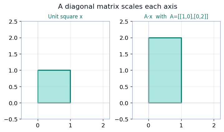
Let \(A=\begin{bmatrix}1&0\\0&2\end{bmatrix}\) (a diagonal scaling matrix) and \(x=\begin{bmatrix}3\\4\end{bmatrix}\).

\[ T(x) = Ax = \begin{bmatrix}1&0\\0&2\end{bmatrix}\begin{bmatrix}3\\4\end{bmatrix} = \begin{bmatrix}1\cdot 3 + 0\cdot 4\\0\cdot 3 + 2\cdot 4\end{bmatrix} = \begin{bmatrix}3\\8\end{bmatrix} \]

The transformation leaves the first component unchanged and doubles the second.

The unit square transformed by the diagonal matrix diag(1,2), stretched to twice its height — A diagonal matrix scales each axis independently: \(\operatorname{diag}(1,2)\) leaves the horizontal axis fixed and doubles the vertical one, stretching the unit square into a \(1\times 2\) rectangle. Every matrix is a geometric transformation of space. *(From the course notes.)*

Vectors

A vector is an ordered list of numerical values. In machine learning it represents data points, feature sets, model parameters, or predictions, and is usually high-dimensional.

Where vectors appear in Machine Learning

Feature vectors — each data sample is a vector of features, e.g. a house as \(x=[\,2100,\ 3,\ 5,\ 10\,]\) (size, rooms, location code, age).
Parameter vectors — model weights, e.g. in linear regression \(y = w\cdot x + b\), the weight vector \(w\) is learned during training.
Embedding vectors — words/sentences mapped to vectors (Word2Vec, GloVe, BERT) that capture meaning, e.g. \(v_{\text{king}}=[\,0.25,\ -0.10,\ 0.5,\ \dots\,]\).
Input / output vectors — e.g. an image flattened into a long vector of pixels.
Gradient vectors — indicate the direction and size of the parameter update needed to minimize the loss function.

Vectors solve systems of equations. The system \(2a+3b=8,\quad 10a+b=13\) is written compactly as a matrix equation:

\[ \begin{bmatrix}2&3\\10&1\end{bmatrix}\begin{bmatrix}a\\b\end{bmatrix} = \begin{bmatrix}8\\13\end{bmatrix} \]

Vector Operations — Addition

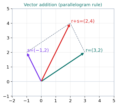
Vectors add component-wise, and geometrically by the parallelogram (tip-to-tail) rule. With \(r=\begin{bmatrix}3\\2\end{bmatrix}\) and \(s=\begin{bmatrix}-1\\2\end{bmatrix}\):

\[ r + s = \begin{bmatrix}3+(-1)\\2+2\end{bmatrix} = \begin{bmatrix}2\\4\end{bmatrix} \]

Vector addition of r and s shown as a parallelogram, with the resultant r plus s — Vector addition as a parallelogram: place the tail of s at the head of r and the diagonal **r + s** is the sum. Addition is commutative, so building the parallelogram the other way gives the same diagonal. *(From the course notes.)*

Multiplication by a scalar

Scaling stretches (\(2r\)), shrinks (\(\tfrac{1}{2}r\)), or reverses (\(-r\)) a vector along the same line:

\[ 2r = \begin{bmatrix}2\cdot 3\\2\cdot 2\end{bmatrix} = \begin{bmatrix}6\\4\end{bmatrix}, \qquad r+(-r) = \begin{bmatrix}3+(-3)\\2+(-2)\end{bmatrix} = \begin{bmatrix}0\\0\end{bmatrix} \]

The dot product

The dot product of two vectors multiplies matching components and sums the results. For \(r=\begin{bmatrix}3\\2\end{bmatrix}\) and \(s=\begin{bmatrix}-1\\2\end{bmatrix}\):

\[ r\cdot s = (3)(-1) + (2)(2) = -3 + 4 = 1 \]

The dot product is the workhorse of deep learning — a single neuron computes the dot product of its inputs with its weights before applying a non-linearity.

Properties

Property	Statement
Commutative (addition)	\(r + s = s + r\)
Associative (addition)	\((r + s) + t = r + (s + t)\)
Commutative (dot product)	\(r \cdot s = s \cdot r\)
Distributive (dot product)	\(r \cdot (s + t) = r \cdot s + r \cdot t\)
Associative over scalar mult.	\(r \cdot (a s) = a(r \cdot s)\)

A worked example for each property. Throughout, use \(r=\begin{bmatrix}3\\2\end{bmatrix},\ s=\begin{bmatrix}-1\\2\end{bmatrix},\ t=\begin{bmatrix}4\\1\end{bmatrix},\) scalar \(a=2\).

Commutative (addition): \(r+s=s+r\)

\[ r+s = \begin{bmatrix}3+(-1)\\2+2\end{bmatrix} = \begin{bmatrix}2\\4\end{bmatrix} = s+r = \begin{bmatrix}-1+3\\2+2\end{bmatrix} = \begin{bmatrix}2\\4\end{bmatrix} \]

Associative (addition): \((r+s)+t=r+(s+t)\)

\[ \underbrace{\begin{bmatrix}2\\4\end{bmatrix}}_{r+s} + \begin{bmatrix}4\\1\end{bmatrix} = \begin{bmatrix}6\\5\end{bmatrix} = \begin{bmatrix}3\\2\end{bmatrix} + \underbrace{\begin{bmatrix}3\\3\end{bmatrix}}_{s+t} = \begin{bmatrix}6\\5\end{bmatrix} \]

Commutative (dot product): \(r\cdot s=s\cdot r\)

\[ r\cdot s = 3(-1)+2(2) = 1 = s\cdot r = (-1)(3)+2(2) = 1 \]

Distributive (dot product): \(r\cdot(s+t)=r\cdot s + r\cdot t\)

\[ r\cdot(s+t) = \begin{bmatrix}3\\2\end{bmatrix}\cdot\begin{bmatrix}3\\3\end{bmatrix} = 9 + 6 = 15 = \underbrace{(r\cdot s)}_{1} + \underbrace{(r\cdot t = 3(4)+2(1))}_{14} = 15 \]

Associative over scalar mult.: \(r\cdot(as)=a(r\cdot s)\)

\[ r\cdot(2s) = \begin{bmatrix}3\\2\end{bmatrix}\cdot\begin{bmatrix}-2\\4\end{bmatrix} = -6 + 8 = 2 = 2(r\cdot s) = 2(1) = 2 \]

Tensors

A tensor is an array of numbers arranged on a grid with any number of axes (dimensions). It is the general object that unifies everything we have seen so far — the number of dimensions is called the tensor's rank.

Dimensions (rank)	Object	Example
0	scalar	\(5\)
1	vector	\(\begin{bmatrix}2 & 3 & -1\end{bmatrix}\)
2	matrix	\(\begin{bmatrix}1&2\\3&4\end{bmatrix}\)
3 or more	higher-order tensor	an RGB image: height × width × channels

Tensors in ML

They are the core data structure of frameworks like PyTorch and TensorFlow. For example, a batch of color images is a 4-D tensor with shape \((\text{batch} \times \text{height} \times \text{width} \times \text{channels})\).

Matrix Multiplication

To multiply \(A\) (\(m\times p\)) by \(B\) (\(p\times n\)), take the dot product of each row of \(A\) with each column of \(B\). The result \(C\) is \(m\times n\), with entries

\[ c_{ij} = \sum_{k} a_{ik}\,b_{kj}. \]

Rule

The inner dimensions must match — \((m\times p)(p\times n) = (m\times n)\).

Worked \(2\times 3\) times \(3\times 2\)

\(A=\begin{bmatrix}1&2&3\\4&5&6\end{bmatrix},\qquad B=\begin{bmatrix}7&8\\9&10\\11&12\end{bmatrix}\)

\[ \begin{aligned} c_{11} &= 1\cdot 7 + 2\cdot 9 + 3\cdot 11 = 7 + 18 + 33 = 58\\ c_{12} &= 1\cdot 8 + 2\cdot 10 + 3\cdot 12 = 8 + 20 + 36 = 64\\ c_{21} &= 4\cdot 7 + 5\cdot 9 + 6\cdot 11 = 28 + 45 + 66 = 139\\ c_{22} &= 4\cdot 8 + 5\cdot 10 + 6\cdot 12 = 32 + 50 + 72 = 154 \end{aligned} \]

\[ C = A\cdot B = \begin{bmatrix}58 & 64\\139 & 154\end{bmatrix} \]

Because the definition uses rows of the left matrix and columns of the right, matrix multiplication is not commutative in general: \(AB \neq BA\).

The Identity Matrix

The identity matrix \(I\) is a square matrix with ones on the main diagonal and zeros elsewhere. It is the multiplicative identity: any matrix multiplied by \(I\) is unchanged. The size is written as a subscript, \(I_n\) for the \(n\times n\) identity.

\[ I_2 = \begin{bmatrix}1&0\\0&1\end{bmatrix}, \quad I_3 = \begin{bmatrix}1&0&0\\0&1&0\\0&0&1\end{bmatrix}, \quad I_4 = \begin{bmatrix}1&0&0&0\\0&1&0&0\\0&0&1&0\\0&0&0&1\end{bmatrix} \]

Properties

Multiplicative identity: for any \(n\times n\) matrix \(A\), \(\ A\,I_n = I_n\,A = A\).
All diagonal elements equal 1.
All non-diagonal elements equal 0.

Multiplying by the identity

For \(A=\begin{bmatrix}2&3\\4&5\end{bmatrix}\):

\[ A\cdot I_2 = \begin{bmatrix}2&3\\4&5\end{bmatrix}\begin{bmatrix}1&0\\0&1\end{bmatrix} = \begin{bmatrix}2\cdot 1 + 3\cdot 0 & 2\cdot 0 + 3\cdot 1\\ 4\cdot 1 + 5\cdot 0 & 4\cdot 0 + 5\cdot 1\end{bmatrix} = \begin{bmatrix}2&3\\4&5\end{bmatrix} \]

Why it matters in ML

The identity matrix is used to initialize parameters. For example, initializing the weights of a recurrent neural network (RNN) with an identity matrix helps stabilize training by keeping gradients from vanishing or exploding early on.

Matrix Inverse & Invertibility

The inverse of a square matrix \(A\), written \(A^{-1}\), is the matrix that "undoes" \(A\):

\[ A^{-1}A = I_n. \]

It is the matrix analogue of dividing by a number. Its main use is solving linear systems.

What "undoes" means

Think of \(A\) as a machine that transforms a vector: put \(x\) in and it returns a moved vector \(Ax\). The inverse \(A^{-1}\) runs that machine backwards — it takes \(Ax\) and returns the original \(x\). Just as multiplying by \(5\) then by \(\tfrac{1}{5}\) leaves a number unchanged, applying \(A\) then \(A^{-1}\) leaves a vector unchanged: \(A^{-1}(Ax) = I_n x = x\). The identity \(I_n\) is the "do-nothing" matrix.

Example

With \(A=\begin{bmatrix}1&2\\3&4\end{bmatrix},\ A^{-1}=\begin{bmatrix}-2&1\\1.5&-0.5\end{bmatrix}\), start from \(x=\begin{bmatrix}1\\1\end{bmatrix}\):

\[ Ax = \begin{bmatrix}3\\7\end{bmatrix} \quad\xrightarrow{\,A^{-1}\,}\quad A^{-1}\begin{bmatrix}3\\7\end{bmatrix} = \begin{bmatrix}-6+7\\4.5-3.5\end{bmatrix} = \begin{bmatrix}1\\1\end{bmatrix} \]

— back to the original vector.

Solving \(Ax=b\)

\[ \begin{aligned} Ax &= b\\ A^{-1}Ax &= A^{-1}b && \text{(left-multiply both sides by } A^{-1})\\ I_n x &= A^{-1}b && \text{(since } A^{-1}A = I_n)\\ x &= A^{-1}b && \text{(since } I_n x = x) \end{aligned} \]

When can a matrix not be inverted?

A matrix is invertible only if it is square and full rank. It has no inverse when:

it has more rows than columns (a tall matrix),
it has more columns than rows (a wide matrix),
it has redundant rows or columns — they are linearly dependent, so the matrix is "low rank".

Inverse of a \(2\times 2\) Matrix

For \(A=\begin{bmatrix}a&b\\c&d\end{bmatrix}\), the inverse (valid only when \(\det A = ad-bc \neq 0\)) is

\[ A^{-1} = \frac{1}{ad-bc}\begin{bmatrix}d&-b\\-c&a\end{bmatrix}. \]

Take \(A=\begin{bmatrix}1&2\\3&4\end{bmatrix}\), so \(\det A = 1\cdot 4 - 2\cdot 3 = -2\):

\[ A^{-1} = \frac{1}{-2}\begin{bmatrix}4&-2\\-3&1\end{bmatrix} = \begin{bmatrix}-2&1\\1.5&-0.5\end{bmatrix} \]

Check:

\[ A^{-1}A = \begin{bmatrix}-2&1\\1.5&-0.5\end{bmatrix}\begin{bmatrix}1&2\\3&4\end{bmatrix} = \begin{bmatrix}1&0\\0&1\end{bmatrix} = I_2, \]

which confirms the result. Row-by-row: \((-2)(1)+(1)(3)=1\), \((-2)(2)+(1)(4)=0\), \((1.5)(1)+(-0.5)(3)=0\), \((1.5)(2)+(-0.5)(4)=1\).

Norms

A norm measures the "size" of a vector — intuitively, its distance from the origin. Formally, the \(L^p\) norm is

\[ \lVert x\rVert_p = \left(\sum_i |x_i|^p\right)^{1/p}, \qquad p\in\mathbb{R},\ p\ge 1. \]

Vector Norms

Norm	Definition	Intuition
1-norm (Manhattan)	\(\lVert x\rVert_1 = \displaystyle\sum_{i=1}^{n} \|x_i\|\)	"total length" of the vector
2-norm (Euclidean)	\(\lVert x\rVert_2 = \sqrt{\displaystyle\sum_{i=1}^{n} \|x_i\|^2}\)	shortest distance from the origin
\(\infty\)-norm (max)	\(\lVert x\rVert_\infty = \displaystyle\max_{1\le i\le n} \|x_i\|\)	largest component in magnitude

Vector norms of \(X=(-1,\ 4,\ 2)\):

\[ \begin{aligned} \lVert X\rVert_1 &= |{-1}| + |4| + |2| = 1 + 4 + 2 = 7\\ \lVert X\rVert_2 &= \sqrt{(-1)^2 + 4^2 + 2^2} = \sqrt{21} \approx 4.58\\ \lVert X\rVert_\infty &= \max(|{-1}|,\ |4|,\ |2|) = 4 \end{aligned} \]

Dot product via norms. \(\ x^\top y = \lVert x\rVert_2\,\lVert y\rVert_2\,\cos\theta\), where \(\theta\) is the angle between \(x\) and \(y\).

Matrix Norms

Norm	Definition	Intuition
1-norm (column-sum)	\(\lVert A\rVert_1 = \displaystyle\max_{1\le j\le n}\sum_{i=1}^{n} \|a_{ij}\|\)	largest column sum
\(\infty\)-norm (row-sum)	\(\lVert A\rVert_\infty = \displaystyle\max_{1\le i\le n}\sum_{j=1}^{n} \|a_{ij}\|\)	largest row sum
Frobenius (2-norm)	\(\lVert A\rVert_F = \sqrt{\displaystyle\sum_{i,j} \|a_{ij}\|^2}\)	entrywise Euclidean length

Matrix 1-norm and \(\infty\)-norm. Let \(A=\begin{bmatrix}7&1&8\\4&5&8\\10&4&2\end{bmatrix}\).

1-norm (sum each column, take the largest):

\[ \lVert A\rVert_1 = \max\big(\underbrace{7+4+10}_{21},\ \underbrace{1+5+4}_{10},\ \underbrace{8+8+2}_{18}\big) = 21 \]

\(\infty\)-norm (sum each row, take the largest):

\[ \lVert A\rVert_\infty = \max\big(\underbrace{7+1+8}_{16},\ \underbrace{4+5+8}_{17},\ \underbrace{10+4+2}_{16}\big) = 17 \]

Eigendecomposition

Just as an integer can be broken into prime factors (\(12 = 2\times 2\times 3\)), a matrix can be decomposed to reveal properties hidden in its array of numbers. Eigendecomposition breaks a matrix into eigenvectors and eigenvalues.

An eigenvector of a square matrix \(A\) is a nonzero vector \(v\) whose direction is unchanged by \(A\) — multiplication only scales it:

\[ Av = \lambda v, \qquad v \neq 0. \]

The scalar \(\lambda\) is the corresponding eigenvalue. If \(v\) is an eigenvector, so is any rescaled \(sv\) (same eigenvalue) — so we usually take unit eigenvectors.

Finding eigenvalues of a \(2\times 2\) matrix

Let \(A=\begin{bmatrix}0&1\\-2&-3\end{bmatrix}\). Solve \(\det(A-\lambda I) = 0\):

\[ \det\begin{bmatrix}-\lambda & 1\\-2 & -3-\lambda\end{bmatrix} = (-\lambda)(-3-\lambda) - (1)(-2) = \lambda^2 + 3\lambda + 2 = 0 \]

\[ (\lambda+1)(\lambda+2) = 0 \ \Rightarrow\ \lambda_1 = -1,\quad \lambda_2 = -2. \]

Each eigenvalue is then substituted back into \((A-\lambda I)v = 0\) to find its eigenvector.

Singular Value Decomposition (SVD)

SVD decomposes any \(m\times n\) matrix into three smaller matrices:

\[ A_{[m\times n]} = U_{[m\times r]}\,\Sigma_{[r\times r]}\,\big(V_{[n\times r]}\big)^{\top} \]

Factor	What it is
\(A\)	input data matrix (\(m\) documents \(\times\) \(n\) terms).
\(U\)	left singular vectors (\(m\) documents \(\times\) \(r\) concepts).
\(\Sigma\)	singular values — diagonal, the strength of each concept (\(r = \text{rank}\)).
\(V\)	right singular vectors (\(n\) terms \(\times\) \(r\) concepts).

The singular values are the square roots of the eigenvalues, sorted in descending order, which makes SVD a core tool for dimensionality reduction.

Full worked SVD of \(A=\begin{bmatrix}1&1\\7&7\end{bmatrix}\)

Step 1 — Form \(AA^\top\) and \(A^\top A\).

\[ AA^\top = \begin{bmatrix}2&14\\14&98\end{bmatrix}, \qquad A^\top A = \begin{bmatrix}50&50\\50&50\end{bmatrix} \]

Step 2 — Eigenvalues (same for both): solve \(\lambda^2 - 100\lambda = 0 \Rightarrow \lambda = 0\) or \(\lambda = 100\).

Step 3 — Left singular vectors \(U\) (eigenvectors of \(AA^\top\), normalized, sorted by \(\lambda\)):

\[ U = \begin{bmatrix}0.14 & -0.99\\0.99 & 0.14\end{bmatrix} \]

Step 4 — Right singular vectors \(V^\top\) (eigenvectors of \(A^\top A\)):

\[ V^\top = \begin{bmatrix}0.70 & 0.70\\-0.70 & 0.70\end{bmatrix} \]

Step 5 — Singular values \(=\sqrt{\lambda}\), largest first:

\[ \Sigma = \begin{bmatrix}\sqrt{100} & 0\\0 & \sqrt{0}\end{bmatrix} = \begin{bmatrix}10 & 0\\0 & 0\end{bmatrix} \]

Result.

\[ \begin{bmatrix}1&1\\7&7\end{bmatrix} = U\Sigma V^\top = \begin{bmatrix}0.14 & -0.99\\0.99 & 0.14\end{bmatrix}\begin{bmatrix}10&0\\0&0\end{bmatrix}\begin{bmatrix}0.70 & 0.70\\-0.70 & 0.70\end{bmatrix} \approx \begin{bmatrix}0.98 & 0.98\\6.93 & 6.93\end{bmatrix} \]

(The small rounding gap comes from using 2-decimal singular vectors.)

Application: Latent Semantic Analysis

Let \(A\) be a documents \(\times\) terms matrix (row per document, column per word). Its SVD reveals hidden topics: \(U\) maps documents \(\to\) concepts, \(V\) maps terms \(\to\) concepts, and the singular values in \(\Sigma\) rank those concepts by importance. Keeping only the top few gives a compact, denoised representation of the corpus. The same machinery underlies PCA and low-rank model compression, where big weight matrices are approximated by the product of two thin ones.

Exercises

Three problems to cement the mechanics. Work each one on paper before opening the solution — the arithmetic is the point.

1

Invert a \(2\times 2\) matrix

Compute the inverse of \(A=\begin{bmatrix}2&1\\7&4\end{bmatrix}\) and verify that \(A^{-1}A = I\).

\[ \det(A) = (2)(4) - (1)(7) = 8 - 7 = 1 \]

\[ A^{-1} = \frac{1}{1}\begin{bmatrix}4&-1\\-7&2\end{bmatrix} = \begin{bmatrix}4&-1\\-7&2\end{bmatrix} \]

\[ A^{-1}A = \begin{bmatrix}4&-1\\-7&2\end{bmatrix}\begin{bmatrix}2&1\\7&4\end{bmatrix} = \begin{bmatrix}1&0\\0&1\end{bmatrix} = I \]

Row-by-row: \((4)(2)+(-1)(7)=1\), \((4)(1)+(-1)(4)=0\), \((-7)(2)+(2)(7)=0\), \((-7)(1)+(2)(4)=1\). Since the determinant is 1, the inverse is just the "swap and negate" pattern with no division: \(A^{-1}=\begin{bmatrix}4&-1\\-7&2\end{bmatrix}\).

2

Frobenius norm

Compute the Frobenius norm of \(\begin{bmatrix}3&4\\0&12\end{bmatrix}\).

\[ \lVert A\rVert_F = \sqrt{3^2 + 4^2 + 0^2 + 12^2} = \sqrt{9 + 16 + 0 + 144} = \sqrt{169} = 13 \]

Square every entry, add them up, take the square root: \(\sqrt{169} = 13\).

3

Matrix \(\times\) vector

Multiply \(\begin{bmatrix}1&2\\3&4\end{bmatrix}\begin{bmatrix}3\\4\end{bmatrix}\) (a \(2\times 2\) matrix times a column vector).

\[ \begin{bmatrix}1&2\\3&4\end{bmatrix}\begin{bmatrix}3\\4\end{bmatrix} = \begin{bmatrix}1\cdot 3 + 2\cdot 4\\3\cdot 3 + 4\cdot 4\end{bmatrix} = \begin{bmatrix}11\\25\end{bmatrix} \]

Each output entry is a row dotted with the vector: row 1 gives \(3+8=11\), row 2 gives \(9+16=25\). Result: \(\begin{bmatrix}11\\25\end{bmatrix}\).

Recap & Where Next

You now know

Scalars scale; vectors are ordered lists (a data point is a vector); matrices and tensors are 2-D and n-D arrays that transform data.
Matrix multiplication is the row-by-column dot product (\(c_{ij}=\sum_k a_{ik}b_{kj}\)); the identity does nothing and the \(2\times 2\) inverse follows a closed-form recipe when \(\det \neq 0\).
Norms summarise size: vector 1-/2-/\(\infty\)-norms, and matrix 1-norm (max column sum), \(\infty\)-norm (max row sum), Frobenius (entrywise Euclidean length).
Eigendecomposition (\(Av=\lambda v\)) and the SVD (\(A = U\Sigma V^\top\)) expose the dominant structure of any matrix and power PCA, LSA and low-rank compression.

Next up: Module 2 — Numerical Computation, where we turn from exact algebra to the realities of finite-precision arithmetic: overflow, underflow, conditioning and gradient-based optimisation — the numerical bedrock on which training actually runs.